At September 2026 rates, the first-year interest on a 90% mortgage for the average home is 77–107% of the rent on that home, and once maintenance, insurance and the return the deposit could have earned are added, owning costs more than renting in all 12 UK regions. Buying comes out ahead through house-price growth: if prices keep rising at their 2005–2026 pace of 3.0% a year, buying beats renting after 1.4 years (Scotland) to 4.1 years (South East); if prices stay flat, it takes 11 years in Scotland, 18–27 years in six other regions and more than 30 years in the other five. Mortgage rates matter almost as much: one percentage point higher stretches the baseline to 2.3–12.2 years. In our 2005–2026 backtest, buyers who sold after five years were ahead of an equivalent renter in 79% of cases, but most who bought in 2006–08 were still behind after five years, and most 2022–24 buyers were behind by 2026. To run your own numbers, use the calculator.
"Renting is dead money" is the most repeated piece of financial advice in Britain. It is half right. Rent buys you nothing you can sell later. But a mortgage is not a savings account either: most of the early payments are interest, and stamp duty, solicitors, surveys, estate agents, repairs and insurance are just as unrecoverable as rent. The honest question is not "rent or own?" but "which set of unrecoverable costs is smaller, for the same home, over the time I will live in it?" We answered it with official data for every UK region and 316 local authorities, and tested the answer against what actually happened to buyers and renters from 2005 to 2026.
In this analysis
- What "dead money" leaves out
- How we compared renting and buying
- Year one: interest versus rent
- Findings by region and property type
- Findings by local authority
- Historical backtest, 2005–2026
- Sensitivity: interest rates, house prices, years held
- What this means if you are deciding
- Limitations
- Reproducible code (Python and R)
- Data downloads
- Frequently asked questions
1. What "dead money" leaves out
The phrase compares the whole of a rent payment with the whole of a mortgage payment and notices that only one of them leaves you owning something. That comparison makes three mistakes. It counts capital repayment as a benefit of buying while ignoring that the deposit used to get the mortgage could have been earning a return instead. It ignores the costs only owners pay: stamp duty (or LBTT in Scotland and LTT in Wales), conveyancing, a survey, mortgage product fees, maintenance, buildings insurance, service charges on flats and, eventually, an estate agent. And it quietly assumes the home will be worth more when you sell it, which is the one part of the calculation nobody can know in advance.
The fair comparison takes one home and two households. One buys it. The other rents the same home and invests the money the buyer put into the deposit and buying costs. Each month, whichever household has the lower housing bill invests the difference, so both spend exactly the same. At any point we can ask who is wealthier: the buyer, with the home's value minus the mortgage still owed and the cost of selling, or the renter, with their investments. The month from which the buyer stays ahead is the break-even point. That is the number this article is about.
2. How we compared renting and buying
The homes. For each of the 12 UK regions and nations we take the average price from the HM Land Registry UK House Price Index for July 2026 (the latest month available) and the average monthly private rent for the same month from the ONS Price Index of Private Rents (PIPR). Both series are published by property type, so we also compare like with like: terraced with terraced, flats with flats. Both are published for local authorities in England and Wales, which gives us 316 local comparisons. We do not report a single "UK average" comparison: the UK average rent is weighted towards the rental stock, which is concentrated in London and cities, while the UK average price is weighted by sales, so their ratio describes no real home.
The money. All amounts are nominal pounds. The main scenario is a first-time buyer with a 10% deposit, paying the Bank of England's average quoted rate for a two-year fixed mortgage at 90% loan-to-value in September 2026 (5.37%), re-fixed every two years with a new product fee, on a 25-year repayment mortgage. We also run a 25% deposit at the 75% LTV rate (5.13%). The renter invests at 5% a year, the Financial Conduct Authority's intermediate projection rate for tax-advantaged products such as ISAs. House prices and rents grow at England's average over July 2005 to July 2026: 3.0% a year for prices and 3.0% a year for rents. That window is the longest both series cover, and it contains a crash, a decade of near-zero interest rates, a pandemic boom and the 2022–23 rate shock. Every one of these assumptions is varied in section 7.
| Assumption | Value | Source |
|---|---|---|
| Purchase price | Average by region and type, July 2026 | HM Land Registry UK HPI full file |
| Rent | Average monthly private rent, July 2026; reset once a year | ONS PIPR, 21 October 2026 release |
| Mortgage rate | 5.37% (90% LTV) / 5.13% (75% LTV), 2-year fixed, Sep 2026 | Bank of England IUMB482 / IUMBV34 |
| Transaction tax | SDLT (England, NI), LBTT (Scotland), LTT (Wales) at October 2026 rates, with first-time buyer relief where it exists | GOV.UK, Revenue Scotland, Welsh Government |
| Conveyancing (buying) | £1,420 freehold house; £1,825 leasehold flat | ClearScore solicitor fees guide, 2026 |
| Survey | £400 at £150k rising to £1,200 at £750k | ClearScore solicitor fees guide, 2026 |
| Mortgage product fee | £1,141 at purchase and every 2-year re-fix | Moneyfacts average fixed-rate fee (Feb 2024 data) |
| Selling costs | Estate agent 1.42% inc. VAT; legal £950 | HomeOwners Alliance, 2026 |
| Maintenance | 1% of value a year (houses); 0.5% (flats) | Common 1% rule of thumb; flats figure is our assumption because the service charge covers communal repairs |
| Buildings insurance | £306 a year (houses) | ABI average buildings-only premium, Q1 2026 |
| Service charge (flats) | £2,405 a year; London £2,801 | Hamptons 2025 Service Charge Index (England & Wales) |
| Fixed costs inflation | 2% a year | Bank of England inflation target |
| Renter's return | 5% a year, tax-free (ISA) | FCA COBS 13 Annex 2 intermediate rate |
| Price and rent growth | 3.0% and 3.0% a year | England, July 2005–July 2026, UK HPI and PIPR |
3. Year one: interest versus rent
Start with the simplest version of the question: in the first year, what does owning cost that you will never get back, and how does it compare with rent? Figure 1 stacks the unrecoverable costs of owning the average home in each region with a 10% deposit: mortgage interest, maintenance and insurance, and the 5% return forgone on the deposit and buying costs. Capital repayment is left out because it comes back as equity.
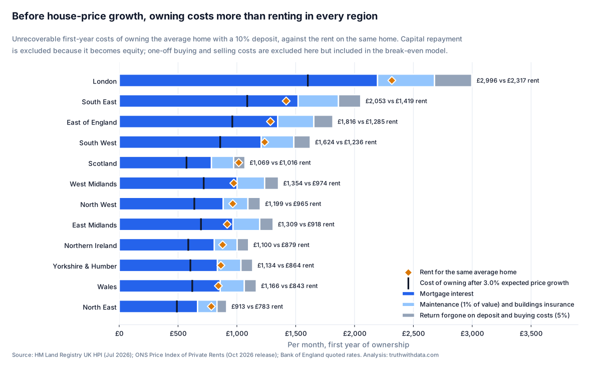
Mortgage interest alone is between 77% of the rent (Scotland) and 107% (South East). In five regions, the East Midlands, West Midlands, East of England, South East and Wales, a first-time buyer's interest bill in year one is larger than the rent they would have paid. Add maintenance, insurance and the forgone return on the deposit and owning costs 5% (Scotland) to 45% (South East) more than renting, everywhere. On these numbers rent is no more "dead" than mortgage interest; it is somewhat less.
What turns the comparison around is the black tick. If the home gains 3.0% in value over the year, that gain, worth more than a year's maintenance and forgone return combined, brings the owner's net cost down to 56–77% of the rent. Buying wins on the expectation of price growth, and on nothing else. Before that growth, it is the more expensive way to live in the same home.
4. Findings by region and property type
A snapshot of one year ignores the upfront costs (which favour renting) and the compounding of price growth on a leveraged asset (which favours buying). The full monthly model handles both. Figure 2 shows the break-even point for the average home in each region under three futures: prices keep rising at 3.0% a year, prices rise at 3.0% but mortgage rates are a point higher (6.37%), and prices stay flat.
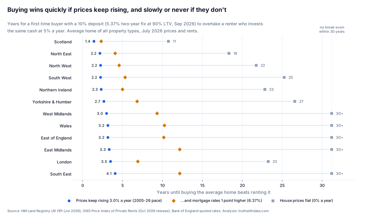
If the next few years look like the last twenty, buying is clearly the better deal in every region for anyone who stays more than about four years, and in most regions after two or three. Scotland is quickest at 1.4 years, because its rents are high relative to prices (a gross yield of 6.2%) and LBTT is low; the South East is slowest at 4.1 years. London's high prices are offset by high rents, putting it at 3.5 years, though its £17,500 stamp duty bill (above the first-time buyer threshold) makes early sale expensive.
The flat-price column is the other half of the story. With no price growth the buyer is relying on equity built by repayments and on rent rising faster than their own costs, and at a 5.37% mortgage rate that takes 11 years in Scotland and 18–27 years in six other regions. In the East Midlands, West Midlands, East of England, South East and Wales, the buyer is still behind after 30 years. The table has the full figures, including the wealth gap after five and ten years.
| Region | Avg price | Rent / month | Gross yield | Tax (FTB) | Break-even: prices +3.0% | Rates +1 pt | Flat prices | Buyer vs renter, 5 yrs | 10 yrs |
|---|---|---|---|---|---|---|---|---|---|
| Scotland | £196,349 | £1,016 | 6.2% | £427 | 1.4 | 2.3 | 10.8 | +£20,691 | +£61,038 |
| North East | £166,943 | £783 | 5.6% | £0 | 2.2 | 4.1 | 18.3 | +£10,915 | +£35,715 |
| South West | £302,298 | £1,236 | 4.9% | £115 | 2.2 | 5.3 | 25.2 | +£13,851 | +£47,068 |
| North West | £221,445 | £965 | 5.2% | £0 | 2.2 | 4.6 | 21.8 | +£12,109 | +£40,268 |
| Northern Ireland | £202,487 | £879 | 5.2% | £0 | 2.3 | 5.0 | 22.8 | +£10,065 | +£34,718 |
| Yorkshire & Humber | £209,116 | £864 | 5.0% | £0 | 2.7 | 6.8 | 26.6 | +£7,544 | +£28,780 |
| West Midlands | £250,880 | £974 | 4.7% | £0 | 3.0 | 9.3 | 30+ | +£6,345 | +£27,120 |
| East of England | £337,518 | £1,285 | 4.6% | £1,876 | 3.2 | 10.2 | 30+ | +£7,480 | +£35,187 |
| Wales | £215,037 | £843 | 4.7% | £0 | 3.2 | 10.2 | 30+ | +£4,747 | +£22,149 |
| East Midlands | £242,274 | £918 | 4.5% | £0 | 3.3 | 12.2 | 30+ | +£4,199 | +£21,635 |
| London | £550,037 | £2,317 | 5.0% | £17,502 | 3.5 | 6.9 | 23.2 | +£15,548 | +£84,104 |
| South East | £380,878 | £1,419 | 4.5% | £4,044 | 4.1 | 12.2 | 30+ | +£4,925 | +£33,438 |
Average home, all property types, July 2026. First-time buyer, 10% deposit, 5.37%. Break-even in years. Tax = SDLT/LBTT/LTT with first-time buyer relief where available. Positive gaps mean the buyer is wealthier.
The regional averages also hide a large difference between property types (table below). Terraced houses break even fastest in every region (median 1.6 years), because they rent for almost as much as semis while costing less to buy. Detached houses are the worst case for buying: a median of 6.8 years, more than 10 years in four regions, and no break-even within 30 years in London or the South East, where detached homes cost £1.17m and £688k but rent for gross yields of 3.0% and 3.4%. Flats come out well despite our service-charge assumption, with a median of 2.3 years.
| Region | Terraced | Semi-detached | Flat | Detached | All types |
|---|---|---|---|---|---|
| Scotland | 1.2 | 1.7 | 1.8 | 3.2 | 1.4 |
| North East | 1.3 | 2.1 | 2.8 | 3.2 | 2.2 |
| South West | 1.3 | 2.2 | 1.6 | 10.6 | 2.2 |
| North West | 1.2 | 2.1 | 2.2 | 6.4 | 2.2 |
| Northern Ireland | 1.3 | 2.2 | 3.0 | 4.8 | 2.3 |
| Yorkshire & Humber | 1.6 | 2.4 | 3.1 | 7.0 | 2.7 |
| West Midlands | 1.7 | 2.6 | 2.4 | 15.2 | 3.0 |
| East of England | 1.7 | 2.8 | 1.7 | 10.2 | 3.2 |
| Wales | 1.7 | 2.8 | 3.1 | 13.4 | 3.2 |
| East Midlands | 1.7 | 2.5 | 2.6 | 6.7 | 3.3 |
| London | 3.2 | 4.2 | 1.8 | 30+ | 3.5 |
| South East | 1.8 | 4.1 | 1.4 | 30+ | 4.1 |
| Median of regions | 1.6 | 2.5 | 2.3 | 8.6 | 2.8 |
Break-even in years by property type, baseline assumptions, 10% deposit. Flats include a service charge and 0.5% maintenance; houses 1% maintenance and buildings insurance.
Using each region's own 2005–2026 price and rent growth instead of England's, the break-even ranges from 0.8 years in Northern Ireland, where prices have risen 5.6% a year since 2015, to 5.3 years in the North East, where prices rose only 1.8% a year from 2005 while rents rose 2.5%. Regional history is not a forecast, which is why we use one common assumption in the main results.
5. Findings by local authority
Regional averages blend cities and countryside with very different rent-to-price ratios. Figure 3 repeats the baseline calculation for the 316 local authorities in England and Wales for which both HM Land Registry and ONS publish July 2026 figures.
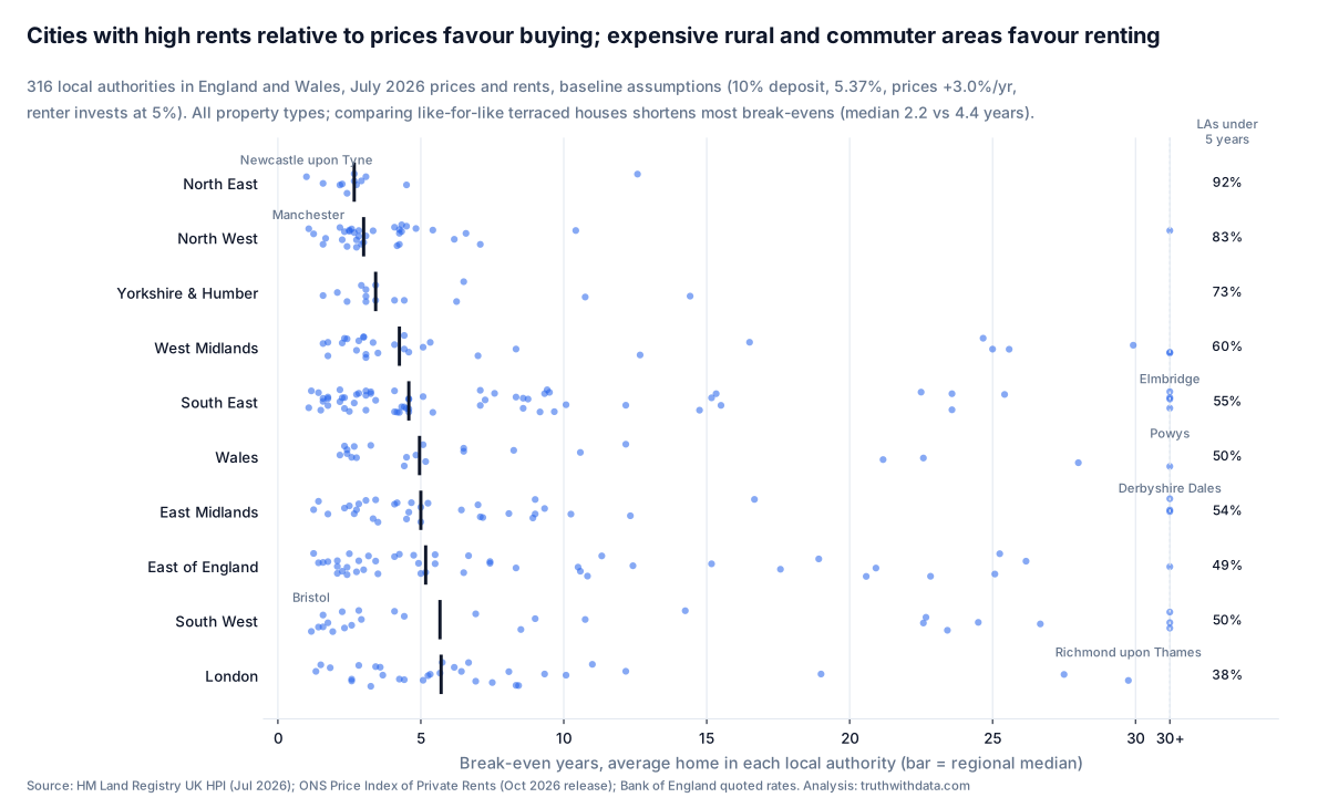
The pattern is driven almost entirely by the gross rental yield, rent as a share of price: across authorities the correlation between yield and break-even is −0.77. In 181 authorities (57%) buying the average home beats renting within five years. In 55 it takes more than ten, and in 15 the buyer is still behind after 30 years. The fastest are cities where rents are high relative to prices: Newcastle upon Tyne (1.0 years, yield 7.0%), Manchester, Portsmouth, Bristol and Southampton (1.1–1.2 years). The 15 that never break even are expensive rural and commuter districts with yields of 2.7–3.5%, including Elmbridge, Waverley and Mole Valley in Surrey, the Derbyshire Dales, South Hams, Malvern Hills and Powys. London spans almost the whole range, from Tower Hamlets (1.3 years) and Newham (1.5) to Kingston upon Thames (19), Kensington and Chelsea (27.5) and Richmond upon Thames (29.75).
Local averages compare different homes
At local authority level the "average home" for sale and the "average home" for rent can be quite different: rented stock in a city is mostly flats and terraces, while sales in a rural district include many detached houses. Comparing like with like reduces the gap. Using terraced houses only, the median break-even across authorities falls from 4.25 to 2.25 years; using flats, also 2.25. The ranking of authorities is similar (rank correlation 0.74), but the all-types figures, especially the "never" cases, are probably biased towards renting.
6. Historical backtest, 2005–2026
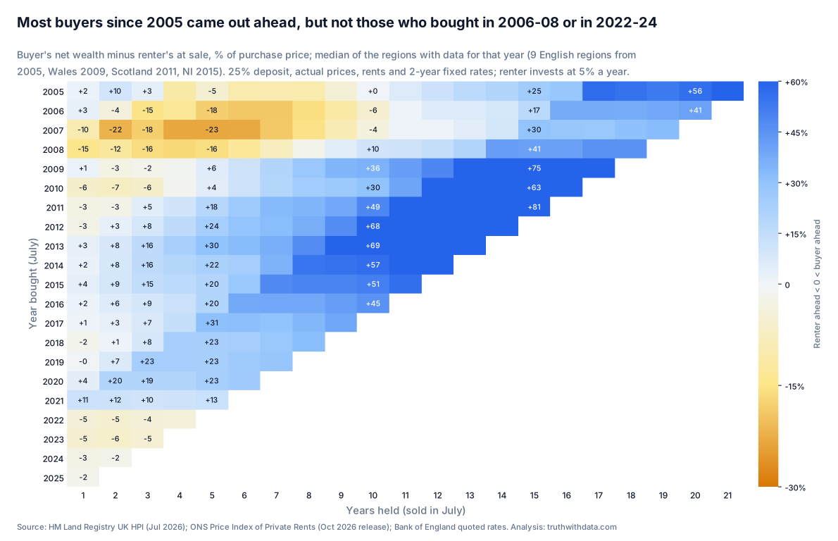
A forecast with one assumed growth rate cannot show what happens when prices fall, rates jump or rents surge. So we replayed history. For every region and every July from 2005 (2009 for Wales, 2011 for Scotland, 2015 for Northern Ireland, when their rent series start) we simulated a buyer and a renter of the region's average home, using the actual monthly prices, actual rents, and the actual 2-year fixed rate at each re-fix. The buyer has a 25% deposit, because the 75% LTV rate series is the only one complete back to 2005. The renter invests either at 5% a year or at Bank Rate, a proxy for the best cash savings rate. That gives 232 purchase dates and 2,418 buy-and-sell pairs in each version.
| Years held | Cases | Buyer ahead (renter earns 5%) | Buyer ahead (renter earns Bank Rate) | Median gap, % of price (5%) |
|---|---|---|---|---|
| 1 year | 232 | 47% | 54% | -0.3% |
| 2 years | 220 | 60% | 64% | +2.4% |
| 3 years | 208 | 68% | 71% | +7.0% |
| 5 years | 184 | 79% | 83% | +17.9% |
| 7 years | 160 | 80% | 87% | +28.1% |
| 10 years | 124 | 86% | 98% | +42.6% |
| 15 years | 67 | 96% | 100% | +51.9% |
| 20 years | 18 | 100% | 100% | +52.7% |
Every region and July purchase date from 2005 to 2025, sold in July of each later year to 2026. 25% deposit, actual prices, rents and 2-year fixed rates (75% LTV).
Three findings stand out. First, buying usually won, and won big over long holds. Holding for five years, the buyer finished ahead in 79% of cases; holding for ten, 86%; and every 20-year hold in the data (18 of them, all England) ended with the buyer ahead. When the renter's alternative is cash at Bank Rate, which was 0.1–0.75% from 2009 to 2021, buying wins even more often: 83% of five-year holds and 98% of ten-year holds.
Second, timing can override everything. A buyer in July 2007 who sold five years later was behind the renter by between 4% of the purchase price (London) and 29% (North East); it took them 6 years (London) to 19 years (North East) to get ahead. Buyers in July 2022, 2023 and 2024 were behind an equivalent renter in 8 of 12 regions by July 2026, by a median of 2–5% of the price: they bought near a price peak, just as mortgage rates jumped.
Third, short holds are close to a coin toss. Selling after one year, the buyer was ahead in 47% of cases, and after two years in 60%. Stamp duty, fees and the estate agent take most of the first year's equity, so short-term outcomes depend on whether prices happened to rise in that particular year.
The backtest flatters buyers in one way
A renter who put the deposit into a global equity fund from 2009 to 2021 would probably have earned considerably more than our 5% assumption, which would shrink the buyer's lead in those years. We do not have a licensed equity index history to test this directly, so we show the 5% and cash versions and say so. Use the calculator to try 7% or 8%.
7. Sensitivity: interest rates, house prices, years held
Every number above rests on assumptions, so we varied each one, running all 12 regions for every combination and reporting the median break-even. Figure 5 crosses the two assumptions that matter most: the mortgage rate and house-price growth.
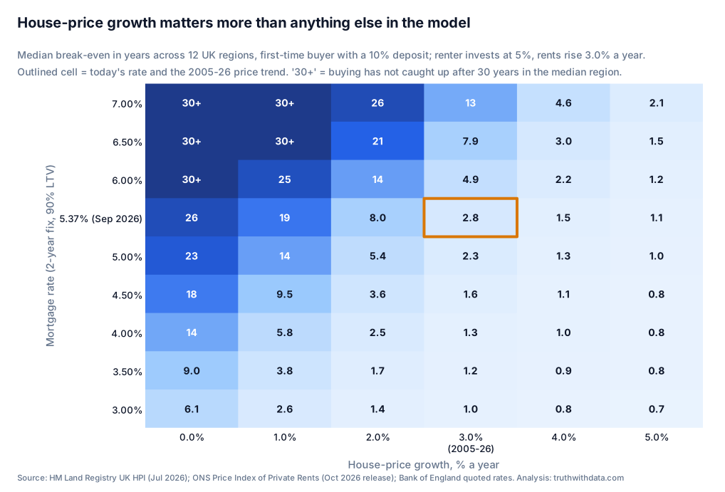
House-price growth dominates. At today's rate, the median break-even goes from 2.8 years with 3.0% growth to 8.0 years with 2%, 19 years with 1% and 26 years with none. No other input moves the answer that much. Interest rates come second. With 3.0% growth, a 4% mortgage rate gives a median break-even of 1.3 years; 6% gives 4.9 years; 7% gives 13. The reason is leverage: with a 10% deposit, the interest rate applies to a loan nine times the size of the buyer's stake.
| Renter's return | Prices 0.0% | Prices 1.0% | Prices 2.0% | Prices 3.0% | Prices 4.0% | Prices 5.0% |
|---|---|---|---|---|---|---|
| 2% | 15.3 | 9.1 | 4.5 | 2.2 | 1.2 | 0.9 |
| 3% | 17.9 | 11.1 | 5.1 | 2.3 | 1.3 | 1.0 |
| 4% | 21.2 | 14.1 | 6.3 | 2.6 | 1.4 | 1.0 |
| 5% (FCA intermediate) | 25.9 | 18.7 | 8.0 | 2.8 | 1.5 | 1.1 |
| 6% | 30+ | 27.5 | 11.8 | 3.2 | 1.6 | 1.1 |
| 7% | 30+ | 30+ | 30+ | 4.1 | 1.7 | 1.2 |
| 8% | 30+ | 30+ | 30+ | 30+ | 2.5 | 1.2 |
Median break-even in years across 12 regions, by the renter's investment return and house-price growth; mortgage rate 5.37%, rents +3.0% a year.
The renter's return matters more than people expect. At 2% (roughly a good cash rate in real terms), the median break-even is 2.2 years; at 8% (the FCA's higher projection rate) the median buyer never stays ahead within 30 years, because the renter's compounding catches up in the later decades. Rent growth matters less when prices are rising: from 1% to 5% a year, the baseline break-even moves only from 3.0 to 2.7 years. It matters a great deal when prices are not rising: with 2% price growth, rents rising 1% a year mean the buyer never catches up, and 5% a year brings break-even down to 5.8 years.
Maintenance and deposit size are secondary. Halving maintenance to 0.5% of value cuts the median break-even from 2.8 to 2.0 years; raising it to 1.5% lifts it to 4.9 (8.3 in the slowest region). A bigger deposit barely matters in the model: 5% gives 2.9 years and 40% gives 2.6. In real life a bigger deposit matters more than this, because it unlocks cheaper rates and smaller monthly payments, and below a 10% deposit many buyers cannot borrow at all.
Years held is the decision you control. The next table shows how much better or worse off the buyer is than the renter after 2, 5, 10 and 20 years in each region, at baseline assumptions. After two years the buyer is behind in 11 of 12 regions, mostly by a few thousand pounds and by £14,400 in London, where stamp duty is largest. After five years the buyer is ahead everywhere; after 20, by £90,000 to £334,000.
| Region | After 2 years | After 5 years | After 10 years | After 20 years |
|---|---|---|---|---|
| Scotland | +£2,313 | +£20,691 | +£61,038 | +£204,965 |
| North East | −£560 | +£10,915 | +£35,715 | +£126,793 |
| South West | −£1,070 | +£13,851 | +£47,068 | +£169,880 |
| North West | −£740 | +£12,109 | +£40,268 | +£144,018 |
| Northern Ireland | −£1,256 | +£10,065 | +£34,718 | +£126,240 |
| Yorkshire & Humber | −£2,226 | +£7,544 | +£28,780 | +£109,048 |
| West Midlands | −£3,116 | +£6,345 | +£27,120 | +£106,947 |
| East of England | −£4,853 | +£7,480 | +£35,187 | +£140,767 |
| Wales | −£3,287 | +£4,747 | +£22,149 | +£89,744 |
| East Midlands | −£3,784 | +£4,199 | +£21,635 | +£90,067 |
| London | −£14,368 | +£15,548 | +£84,104 | +£334,328 |
| South East | −£7,631 | +£4,925 | +£33,438 | +£143,190 |
Buyer's net wealth minus renter's, nominal pounds, baseline assumptions, average home, 10% deposit. Negative = the renter is ahead.
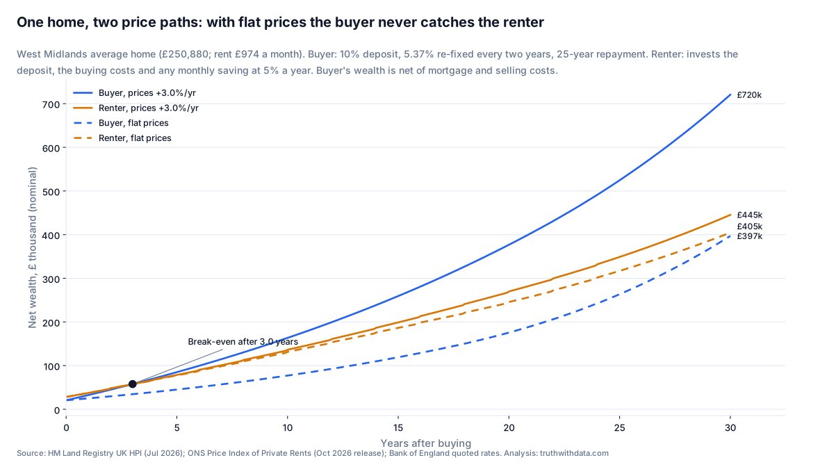
Figure 6 shows why a single break-even figure can mislead. With 3.0% growth the buyer overtakes after three years and, after 30, is worth £720,000 against the renter's £445,000. With flat prices the same purchase leaves the buyer slightly behind the renter for all 30 years, ending at £397,000 against £405,000. The renter's outcome barely changes between the two scenarios; the buyer's depends almost entirely on prices.
8. What this means if you are deciding
Rent is not dead money, and neither is buying a sure thing. Rent pays for somewhere to live with no maintenance bills, no transaction costs and the freedom to move. Mortgage interest pays for the same thing plus a leveraged bet on house prices. Over the last 20 years that bet mostly paid off. Whether it pays off for you depends on three things, in this order:
- How long you will stay. Under two years, buying usually loses: our backtest gives the buyer roughly a coin-toss chance over one to two years, and the forward model has the buyer behind after two years in 11 of 12 regions. Beyond five years, buying won in 79% of historical cases and wins in every region at baseline assumptions.
- What happens to house prices. If you think prices will roughly track the last 20 years, buying wins quickly almost everywhere. If you think they will stagnate, buying takes decades to win, or never does, at today's rates.
- The local rent-to-price ratio. Where rents are high relative to prices, in most cities and for terraced houses and flats, buying wins faster. In expensive rural and commuter areas and for detached houses, renting is often the cheaper way to live in the same home.
One part of the "dead money" argument is right, and it is behavioural: the model assumes the renter actually invests the deposit and every month's saving. A renter who spends that money instead ends up with nothing, and a mortgage is a form of forced saving. If you rent, the comparison only holds if you automate the investing.
Run the numbers for your own home
Our free Rent vs Buy Calculator starts from the July 2026 average price and rent for your region and property type, applies the right stamp duty, LBTT or LTT, and lets you change every assumption. It shows your break-even year, net wealth over 30 years and a plain-English verdict. It runs entirely in your browser.
Affiliate placeholder 1 — partner link to be added (for example, a mortgage broker).
Disclosure: some links on this page may be affiliate links. If you use them we may earn a commission, at no extra cost to you. It never affects our analysis, which was finished before any partner was chosen.
Affiliate placeholder 2 — partner link to be added (for example, a Stocks and Shares ISA platform).
Disclosure: affiliate link. Capital at risk; investments can fall as well as rise.
9. Limitations
- Averages are not homes. Our prices are averages of homes sold and our rents averages of homes let. The two populations differ in size, age and location, most of all at local authority level. Comparing by property type narrows the gap but does not close it.
- The forward model uses one constant growth rate. Real prices move in cycles, and the backtest shows that the year you buy can matter more than the average. The constant mortgage rate is equally unrealistic; it is a scenario, not a forecast.
- Tax is simplified. We assume the renter's investments sit in an ISA and are tax-free. The ISA allowance is £20,000 a year, so a London deposit (£55,000) would take three tax years to shelter; outside an ISA, taxes on returns would favour buying. The backtest applies today's stamp duty rules to past purchases, which understates the stamp duty most buyers actually paid before 2014.
- Some assumptions are thinly sourced. The 1%-of-value maintenance rule is a rule of thumb, not a measured average, and it may overstate maintenance where land is a large share of value (London). Service charges come from one estate agency's index for England and Wales and are applied to Scotland and Northern Ireland too. The product fee figure dates from February 2024. Each is varied or editable in the calculator.
- Mortgage rates. Bank of England quoted rates are averages of advertised rates, not what any individual is offered. The 90% LTV series starts only in 2008 and has gaps, so the backtest uses 75% LTV. We had only 2-year fixed rates; many buyers choose 5-year fixes.
- Not included: moving costs, furnishing, ground rent, leasehold extensions, the cost of a renter being asked to leave, rent controls, government schemes, mortgage-free years after the 25-year term (they fall outside most horizons) and anything non-financial: security, control over the home, flexibility. The model counts money, not wellbeing.
- Northern Ireland prices are quarterly and its rents lag by two months; Scotland's rents are not published at council level, so it is missing from the local analysis.
10. Reproducible code (Python and R)
The analysis was done in Python and independently re-implemented in R from the published CSVs. The R script reproduces every regional break-even exactly (all 120 region × property type × deposit cases agree to the month) and every backtest share. The calculator's JavaScript was checked against the same 120 cases. The Python script reads the four source files exactly as downloaded; the R script needs only base R.
Download: uk-rent-vs-buy-analysis.py (analysis) and uk-rent-vs-buy-charts.py (charts). Run with python uk-rent-vs-buy-analysis.py RAW_DIR OUT_DIR.
Show the full Python analysis script
#!/usr/bin/env python3
"""
Is renting really 'dead money' in the UK?  Truth with Data, October 2026.
Rent-versus-buy model: break-even years by region and local authority,
a historical backtest (2005-2026) and sensitivity tables.

Usage:
    pip install pandas numpy openpyxl
    python uk-rent-vs-buy-analysis.py RAW_DIR OUT_DIR

RAW_DIR must contain the four source files exactly as downloaded:
    UK-HPI-full-file-2026-07.csv                          HM Land Registry, UK HPI (July 2026 data)
    priceindexofprivaterentsukmonthlypricestatistics.xlsx ONS PIPR, 21 October 2026 edition
    priceindexofprivaterentsukhistoricalseries.xlsx       ONS PIPR historical series, 26 March 2025
    Bank_of_England__Database.xlsx                        BoE quoted 2-year fixed mortgage rates
                                                          (IUMBV34, IUMB482, ...), monthly, 1995-2026

The model (identical in the R script):
  * The buyer pays a deposit plus buying costs. The renter keeps that same cash
    invested instead.
  * Every month, whoever has the lower housing outgoings invests the difference.
    Buyer outgoings: mortgage payment (interest + capital), maintenance,
    buildings insurance, service charge (flats), a product fee at each 2-year re-fix.
    Renter outgoings: rent, re-set once a year.
  * Buyer net wealth = home value - mortgage balance - selling costs + buyer's investments.
    Renter net wealth = renter's investments.
  * Break-even = first month from which the buyer's net wealth stays ahead of the renter's.
Capital repayment is not a cost: it reappears as equity. What the buyer loses is
interest, maintenance, insurance, fees, taxes and the return the cash would
have earned; what the buyer gains is house-price growth.
"""
import sys, os, json
import numpy as np
import pandas as pd

RAW = sys.argv[1] if len(sys.argv) > 1 else "raw"
OUT = sys.argv[2] if len(sys.argv) > 2 else "out"
os.makedirs(OUT, exist_ok=True)

# ---------------------------------------------------------------------------
# 1. Assumptions (every number has a source; see the article's methodology)
# ---------------------------------------------------------------------------
A = dict(
    ref_month="2026-07-01",          # latest UK HPI month; PIPR rents for the same month
    rate_month="2026-09-30",         # latest BoE quoted rate (what a buyer pays today)
    term_years=25,                   # repayment mortgage term
    fix_months=24,                   # 2-year fixes, re-fixed at the same rate in the forward model
    product_fee=1141.0,              # Moneyfacts average fixed-rate product fee (Feb 2024)
    conveyancing_house=1420.0,       # ClearScore 2026 guide: freehold purchase, fees + disbursements
    conveyancing_flat=1825.0,        # same guide: leasehold flat £1,550-£2,100 (midpoint)
    survey_points=[(150000, 400), (250000, 600), (400000, 800), (750000, 1200)],  # same guide
    agent_fee_pct=1.42,              # HomeOwners Alliance 2026 average, inc. VAT
    conveyancing_sell=950.0,         # HomeOwners Alliance: £610-£950 to sell (upper end)
    maintenance_house_pct=1.0,       # widely used 1%-of-value rule of thumb (sensitivity 0.5-1.5%)
    maintenance_flat_pct=0.5,        # our assumption: the service charge covers communal repairs
    buildings_insurance=306.0,       # ABI average buildings-only premium, Q1 2026 (houses only)
    service_charge_ew=2405.0,        # Hamptons 2025 Service Charge Index, England & Wales average
    service_charge_london=2801.0,    # Hamptons 2025, London
    cost_inflation_pct=2.0,          # fixed £ costs grow at the Bank of England's 2% CPI target
    invest_return_pct=5.0,           # FCA COBS 13 Annex 2 intermediate projection rate (ISA wrapper)
    invest_low_pct=2.0, invest_high_pct=8.0,
    horizon_years=30,
)

REGIONS = [  # (display name, ONS/HMLR code, nation for transaction tax)
    ("North East", "E12000001", "england"), ("North West", "E12000002", "england"),
    ("Yorkshire and The Humber", "E12000003", "england"), ("East Midlands", "E12000004", "england"),
    ("West Midlands", "E12000005", "england"), ("East of England", "E12000006", "england"),
    ("London", "E12000007", "england"), ("South East", "E12000008", "england"),
    ("South West", "E12000009", "england"), ("Wales", "W92000004", "wales"),
    ("Scotland", "S92000003", "scotland"), ("Northern Ireland", "N92000002", "ni"),
]
# No "UK average" row: the UK average rent is weighted by the rental stock (London-heavy) and the
# UK average price by sales, so their ratio describes no real home. We compare like with like by region.
TYPES = {  # model type: (HPI price column, PIPR rent column)
    "all": ("AveragePrice", "Rental price"),
    "detached": ("DetachedPrice", "Rental price detached"),
    "semi": ("SemiDetachedPrice", "Rental price semidetached"),
    "terraced": ("TerracedPrice", "Rental price terraced"),
    "flat": ("FlatPrice", "Rental price flat maisonette"),
}

# Bank Rate changes since 2004 (Bank of England, "Official Bank Rate history").
BANK_RATE = [("2004-02-05", 4.00), ("2004-05-06", 4.25), ("2004-06-10", 4.50), ("2004-08-05", 4.75),
             ("2005-08-04", 4.50), ("2006-08-03", 4.75), ("2006-11-09", 5.00), ("2007-01-11", 5.25),
             ("2007-05-10", 5.50), ("2007-07-05", 5.75), ("2007-12-06", 5.50), ("2008-02-07", 5.25),
             ("2008-04-10", 5.00), ("2008-10-08", 4.50), ("2008-11-06", 3.00), ("2008-12-04", 2.00),
             ("2009-01-08", 1.50), ("2009-02-05", 1.00), ("2009-03-05", 0.50), ("2016-08-04", 0.25),
             ("2017-11-02", 0.50), ("2018-08-02", 0.75), ("2020-03-11", 0.25), ("2020-03-19", 0.10),
             ("2021-12-16", 0.25), ("2022-02-03", 0.50), ("2022-03-17", 0.75), ("2022-05-05", 1.00),
             ("2022-06-16", 1.25), ("2022-08-04", 1.75), ("2022-09-22", 2.25), ("2022-11-03", 3.00),
             ("2022-12-15", 3.50), ("2023-02-02", 4.00), ("2023-03-23", 4.25), ("2023-05-11", 4.50),
             ("2023-06-22", 5.00), ("2023-08-03", 5.25), ("2024-08-01", 5.00), ("2024-11-07", 4.75),
             ("2025-02-06", 4.50), ("2025-05-08", 4.25), ("2025-08-07", 4.00), ("2025-12-18", 3.75)]

# ---------------------------------------------------------------------------
# 2. Transaction taxes in force in October 2026
# ---------------------------------------------------------------------------
def banded(price, bands):
    """bands: list of (upper threshold, rate %) applied to the slice below each threshold."""
    tax, lower = 0.0, 0.0
    for upper, rate in bands:
        if price > lower:
            tax += (min(price, upper) - lower) * rate / 100
        lower = upper
    return tax

INF = float("inf")
SDLT = [(125000, 0), (250000, 2), (925000, 5), (1500000, 10), (INF, 12)]           # England & NI
SDLT_FTB = [(300000, 0), (500000, 5)]                                                 # price <= £500k
LBTT = [(145000, 0), (250000, 2), (325000, 5), (750000, 10), (INF, 12)]               # Scotland
LBTT_FTB = [(175000, 0), (250000, 2), (325000, 5), (750000, 10), (INF, 12)]
LTT = [(225000, 0), (400000, 6), (750000, 7.5), (1500000, 10), (INF, 12)]             # Wales, no FTB relief

def transaction_tax(price, nation, first_time_buyer=True):
    if nation in ("england", "ni"):
        if first_time_buyer and price <= 500000:
            return banded(price, SDLT_FTB)
        return banded(price, SDLT)
    if nation == "scotland":
        return banded(price, LBTT_FTB if first_time_buyer else LBTT)
    if nation == "wales":
        return banded(price, LTT)
    raise ValueError(nation)

def survey_cost(price):
    xs, ys = zip(*A["survey_points"])
    return float(np.interp(price, xs, ys))

# ---------------------------------------------------------------------------
# 3. The model: one monthly simulation gives buyer and renter wealth at every horizon
# ---------------------------------------------------------------------------
def simulate(value, rent, mrate, ret, cidx, deposit_pct, nation, is_flat, region_code,
             ftb=True, maint_pct=None):
    """value[m], cidx[m] for m = 0..M; rent[m], ret[m] for m = 1..M (rent[0], ret[0] unused);
    mrate[m] = quoted 2-year fixed rate (%) available at the end of month m.
    Returns (buyer_wealth, renter_wealth) arrays of length M+1."""
    M = len(value) - 1
    P = value[0]
    if maint_pct is None:
        maint_pct = A["maintenance_flat_pct"] if is_flat else A["maintenance_house_pct"]
    sc = 0.0
    if is_flat:
        sc = A["service_charge_london"] if region_code == "E12000007" else A["service_charge_ew"]
    ins = 0.0 if is_flat else A["buildings_insurance"]
    conv = A["conveyancing_flat"] if is_flat else A["conveyancing_house"]

    deposit = P * deposit_pct / 100
    loan = P - deposit
    buy_costs = transaction_tax(P, nation, ftb) + (conv + A["product_fee"]) * cidx[0] + survey_cost(P)
    renter = deposit + buy_costs          # the renter invests the cash the buyer spends up front
    buyer = 0.0                           # buyer's side pot (invested when owning is cheaper)
    bal, n_left = loan, A["term_years"] * 12
    i = mrate[0] / 1200
    pmt = bal * i / (1 - (1 + i) ** -n_left)

    def sell_cost(v, c):
        return v * A["agent_fee_pct"] / 100 + A["conveyancing_sell"] * c

    bw = np.empty(M + 1); rw = np.empty(M + 1)
    bw[0] = value[0] - bal - sell_cost(value[0], cidx[0]); rw[0] = renter
    for m in range(1, M + 1):
        g = (1 + ret[m] / 100) ** (1 / 12)
        renter *= g; buyer *= g
        pay = 0.0
        if bal > 0:
            interest = bal * i
            principal = min(pmt - interest, bal)
            pay = interest + principal
            bal -= principal; n_left -= 1
            if bal < 1e-6:
                bal = 0.0
        out = pay + maint_pct / 100 * value[m - 1] / 12 + (ins + sc) / 12 * cidx[m]
        if m % A["fix_months"] == 0 and bal > 0 and m < M:   # re-fix: new rate, product fee
            i = mrate[m] / 1200
            pmt = bal * i / (1 - (1 + i) ** -n_left)
            out += A["product_fee"] * cidx[m]
        diff = out - rent[m]
        if diff > 0:
            renter += diff
        else:
            buyer -= diff
        bw[m] = value[m] - bal - sell_cost(value[m], cidx[m]) + buyer
        rw[m] = renter
    return bw, rw

def breakeven_years(bw, rw):
    """Break-even in years: the first month from which the buyer stays ahead of the renter for the
    rest of the horizon (NaN if the buyer is behind at the end). Using the last crossing rather than
    the first stops a brief lead (e.g. just before a re-fix fee or a price fall) counting as break-even."""
    behind = np.nonzero(bw[1:] < rw[1:])[0]
    if len(behind) == 0:
        return 1 / 12
    if behind[-1] == len(bw) - 2:
        return np.nan
    return (behind[-1] + 2) / 12

def forward_paths(P, R0, rate_pct, g_price, g_rent, r_inv, years=None):
    years = years or A["horizon_years"]
    M = years * 12
    m = np.arange(M + 1)
    value = P * (1 + g_price / 100) ** (m / 12)
    rent = R0 * (1 + g_rent / 100) ** ((m - 1) // 12)          # tenancy re-set once a year
    mrate = np.full(M + 1, rate_pct)
    ret = np.full(M + 1, r_inv)
    cidx = (1 + A["cost_inflation_pct"] / 100) ** (m / 12)
    return value, rent, mrate, ret, cidx

def run_forward(P, R0, rate_pct, g_price, g_rent, r_inv, deposit_pct, nation, is_flat, code, **kw):
    v, r, mr, rt, c = forward_paths(P, R0, rate_pct, g_price, g_rent, r_inv)
    return simulate(v, r, mr, rt, c, deposit_pct, nation, is_flat, code, **kw)

# ---------------------------------------------------------------------------
# 4. Load data
# ---------------------------------------------------------------------------
hpi = pd.read_csv(os.path.join(RAW, "UK-HPI-full-file-2026-07.csv"), low_memory=False)
hpi["Date"] = pd.to_datetime(hpi["Date"], dayfirst=True)

pipr = pd.read_excel(os.path.join(RAW, "priceindexofprivaterentsukmonthlypricestatistics.xlsx"),
                     sheet_name="Table 1", header=2)
pipr["Time period"] = pd.to_datetime(pipr["Time period"])
for c in pipr.columns[4:]:
    pipr[c] = pd.to_numeric(pipr[c], errors="coerce")       # '[x]' (not available) -> NaN

hist = pd.read_excel(os.path.join(RAW, "priceindexofprivaterentsukhistoricalseries.xlsx"),
                     sheet_name="Table 1", header=2)
hist = hist[hist.iloc[:, 0] != "Region Code"].copy()
hist.columns = ["date"] + list(hist.columns[1:])
hist["date"] = pd.to_datetime(hist["date"])
hist_codes = {"North East": "E12000001", "North West": "E12000002", "Yorkshire and The Humber": "E12000003",
              "East Midlands": "E12000004", "West Midlands": "E12000005", "East ": "E12000006",
              "London": "E12000007", "South East": "E12000008", "South West": "E12000009",
              "Wales": "W92000004", "Scotland": "S92000003", "Northern Ireland": "N92000002",
              "England": "E92000001", "United Kingdom": "K02000001"}

boe = pd.read_excel(os.path.join(RAW, "Bank_of_England__Database.xlsx"), header=1)
boe.columns = ["date"] + [str(c).split()[-1] for c in boe.columns[1:]]   # series codes
boe["date"] = pd.to_datetime(boe["date"], format="%d %b %y")
for c in boe.columns[1:]:
    boe[c] = pd.to_numeric(boe[c], errors="coerce")
boe = boe.sort_values("date")
boe["month"] = boe["date"].dt.to_period("M").dt.to_timestamp()
rate_row = boe[boe["date"] == A["rate_month"]].iloc[0]
RATE90, RATE75 = float(rate_row["IUMB482"]), float(rate_row["IUMBV34"])

ref = pd.Timestamp(A["ref_month"])

def rent_index(code):
    """PIPR index (Jan 2023 = 100): historical series before 2015, monthly series from Jan 2015.
    The two are identical where they overlap (checked: 2015-01 to 2025-02)."""
    mon = pipr[pipr["Area code"] == code].set_index("Time period")["Index"].dropna()
    name = [k for k, v in hist_codes.items() if v == code]
    if name:
        h = pd.to_numeric(hist.set_index("date")[name[0]], errors="coerce").dropna()
        return pd.concat([h[h.index < mon.index.min()], mon])
    return mon

# Baseline forward growth: England, July 2005 -> July 2026 (the longest window both series cover)
eng_p = hpi[hpi.AreaCode == "E92000001"].set_index("Date")["AveragePrice"]
eng_r = rent_index("E92000001")
yrs = 21
G_PRICE = float(((eng_p[ref] / eng_p[pd.Timestamp("2005-07-01")]) ** (1 / yrs) - 1) * 100)
G_RENT = float(((eng_r[ref] / eng_r[pd.Timestamp("2005-07-01")]) ** (1 / yrs) - 1) * 100)
uk_p = hpi[hpi.AreaCode == "K02000001"].set_index("Date")["AveragePrice"]
G_PRICE_1995 = float(((uk_p[ref] / uk_p[pd.Timestamp("1995-07-01")]) ** (1 / 31) - 1) * 100)

# ---------------------------------------------------------------------------
# 5. Inputs and break-even by region x property type x deposit
# ---------------------------------------------------------------------------
def region_own_growth(code):
    """Region's own annualised price and rent growth over the longest common window to July 2026."""
    ri = rent_index(code)
    p = hpi[hpi.AreaCode == code].set_index("Date")["AveragePrice"]
    start = max(pd.Timestamp("2005-07-01"), ri.index.min())
    start = pd.Timestamp(year=start.year + (start.month > 7), month=7, day=1)
    n = (ref.year - start.year)
    return (float(((p[ref] / p[start]) ** (1 / n) - 1) * 100),
            float(((ri[ref] / ri[start]) ** (1 / n) - 1) * 100), start.year)

rows = []
for name, code, nation in REGIONS:
    hrow = hpi[(hpi.AreaCode == code) & (hpi.Date == ref)].iloc[0]
    prow = pipr[(pipr["Area code"] == code) & (pipr["Time period"] == ref)].iloc[0]
    gp_own, gr_own, gstart = region_own_growth(code)
    for t, (pc, rc) in TYPES.items():
        P, R0 = float(hrow[pc]), float(prow[rc])
        is_flat = t == "flat"
        for dep, rate in ((10, RATE90), (25, RATE75)):
            bw, rw = run_forward(P, R0, rate, G_PRICE, G_RENT, A["invest_return_pct"], dep, nation, is_flat, code)
            bwo, rwo = run_forward(P, R0, rate, gp_own, gr_own, A["invest_return_pct"], dep, nation, is_flat, code)
            bwf, rwf = run_forward(P, R0, rate, 0.0, G_RENT, A["invest_return_pct"], dep, nation, is_flat, code)
            bwr, rwr = run_forward(P, R0, rate + 1, G_PRICE, G_RENT, A["invest_return_pct"], dep, nation, is_flat, code)
            rows.append(dict(
                region=name, area_code=code, nation=nation, property_type=t, deposit_pct=dep,
                mortgage_rate_pct=rate, price_jul2026=P, monthly_rent_jul2026=R0,
                gross_rental_yield_pct=round(12 * R0 / P * 100, 2),
                price_to_annual_rent=round(P / (12 * R0), 1),
                transaction_tax=round(transaction_tax(P, nation, True)),
                breakeven_years=breakeven_years(bw, rw),
                gap_after_2y=bw[24] - rw[24], gap_after_5y=bw[60] - rw[60],
                gap_after_10y=bw[120] - rw[120], gap_after_20y=bw[240] - rw[240],
                own_growth_price_pct=round(gp_own, 2), own_growth_rent_pct=round(gr_own, 2),
                own_growth_from=gstart, breakeven_years_own_growth=breakeven_years(bwo, rwo),
                breakeven_years_flat_prices=breakeven_years(bwf, rwf),
                breakeven_years_rate_plus_1pt=breakeven_years(bwr, rwr),
            ))
reg = pd.DataFrame(rows)

# First-year snapshot of the unrecoverable cost of owning vs renting (all property types, 10% deposit)
snap = []
for name, code, nation in REGIONS:
    r = reg[(reg.region == name) & (reg.property_type == "all") & (reg.deposit_pct == 10)].iloc[0]
    P, R0 = r.price_jul2026, r.monthly_rent_jul2026
    loan = 0.9 * P; i = RATE90 / 1200; n = A["term_years"] * 12
    pmt = loan * i / (1 - (1 + i) ** -n)
    bal, interest = loan, 0.0
    for _ in range(12):
        it = bal * i; interest += it; bal -= pmt - it
    cash_in = 0.1 * P + r.transaction_tax + A["conveyancing_house"] + A["product_fee"] + survey_cost(P)
    snap.append(dict(region=name, rent_year1=12 * R0, interest=interest,
                     maintenance=A["maintenance_house_pct"] / 100 * P, insurance=A["buildings_insurance"],
                     opportunity_cost=cash_in * A["invest_return_pct"] / 100,
                     expected_price_gain=P * G_PRICE / 100,
                     one_off_buy_and_sell_costs=cash_in - 0.1 * P + P * A["agent_fee_pct"] / 100 + A["conveyancing_sell"]))
snap = pd.DataFrame(snap)
snap["net_cost_of_owning"] = snap[["interest", "maintenance", "insurance", "opportunity_cost"]].sum(axis=1) - snap["expected_price_gain"]

# ---------------------------------------------------------------------------
# 6. Sensitivity: each cell is run for all 12 regions (average home, 10% deposit unless
#    stated); we report the median break-even across regions and the fastest/slowest region.
# ---------------------------------------------------------------------------
base = reg[(reg.property_type == "all") & (reg.deposit_pct == 10)]
sens = []
def add(table, **kw):
    args = dict(rate=RATE90, gp=G_PRICE, gr=G_RENT, ret=A["invest_return_pct"], dep=10, maint=None)
    args.update(kw)
    be, g10 = [], []
    for _, r in base.iterrows():
        bw, rw = run_forward(r.price_jul2026, r.monthly_rent_jul2026, args["rate"], args["gp"], args["gr"],
                             args["ret"], args["dep"], r.nation, False, r.area_code, maint_pct=args["maint"])
        be.append(breakeven_years(bw, rw)); g10.append(bw[120] - rw[120])
    be = np.array(be)
    sens.append(dict(table=table, mortgage_rate_pct=args["rate"], price_growth_pct=args["gp"],
                     rent_growth_pct=args["gr"], invest_return_pct=args["ret"], deposit_pct=args["dep"],
                     maintenance_pct=args["maint"] if args["maint"] is not None else A["maintenance_house_pct"],
                     median_breakeven_years=float(np.median(np.where(np.isnan(be), np.inf, be))),
                     fastest_region_years=float(np.nanmin(be)) if np.isfinite(be).any() else np.nan,
                     slowest_region_years=float(np.max(np.where(np.isnan(be), np.inf, be))),
                     regions_not_breaking_even_in_30y=int(np.isnan(be).sum()),
                     median_gap_after_10y=float(np.median(g10))))
GP_GRID = [0.0, 1.0, 2.0, round(G_PRICE, 2), 4.0, 5.0]       # 3% replaced by the 2005-2026 baseline
for rate in [3.0, 3.5, 4.0, 4.5, 5.0, RATE90, 6.0, 6.5, 7.0]:  # 5.5% replaced by today's 90% LTV rate
    for gp in GP_GRID:
        add("rate_x_price_growth", rate=rate, gp=gp)
for ret in [2.0, 3.0, 4.0, 5.0, 6.0, 7.0, 8.0]:
    for gp in GP_GRID:
        add("return_x_price_growth", ret=ret, gp=gp)
for gr in [1.0, 2.0, round(G_RENT, 2), 4.0, 5.0]:
    for gp in GP_GRID:
        add("rent_growth_x_price_growth", gr=gr, gp=gp)
for maint in [0.5, 1.0, 1.5]:
    add("maintenance", maint=maint)
for dep in [5, 10, 15, 20, 25, 40]:
    add("deposit", dep=dep)
sens = pd.DataFrame(sens).replace(np.inf, np.nan)

# ---------------------------------------------------------------------------
# 7. Local authorities (England and Wales: PIPR and UK HPI share LA codes)
# ---------------------------------------------------------------------------
la_rent = pipr[(pipr["Time period"] == ref) & pipr["Area code"].str.match(r"^(E06|E07|E08|E09|W06)")]
la_rows = []
for _, pr in la_rent.iterrows():
    h = hpi[(hpi.AreaCode == pr["Area code"]) & (hpi.Date == ref)]
    if h.empty or pd.isna(pr["Rental price"]):
        continue
    P, R0 = float(h.iloc[0]["AveragePrice"]), float(pr["Rental price"])
    nation = "wales" if pr["Area code"].startswith("W") else "england"
    bw, rw = run_forward(P, R0, RATE90, G_PRICE, G_RENT, A["invest_return_pct"], 10, nation, False, pr["Area code"])
    row = dict(area_code=pr["Area code"], local_authority=pr["Area name"],
               region=pr["Region or country name"], price_jul2026=P, monthly_rent_jul2026=R0,
               gross_rental_yield_pct=round(12 * R0 / P * 100, 2),
               breakeven_years=breakeven_years(bw, rw),
               gap_after_5y=round(bw[60] - rw[60]), gap_after_10y=round(bw[120] - rw[120]))
    # Robustness: like-for-like by property type (terraced houses, flats) where both series exist
    for t in ("terraced", "flat"):
        pc, rc = TYPES[t]
        Pt, Rt = h.iloc[0][pc], pr[rc]
        if pd.notna(Pt) and pd.notna(Rt):
            bt_, rt_ = run_forward(float(Pt), float(Rt), RATE90, G_PRICE, G_RENT, A["invest_return_pct"], 10,
                                   nation, t == "flat", pr["Area code"])
            row[f"breakeven_years_{t}"] = breakeven_years(bt_, rt_)
        else:
            row[f"breakeven_years_{t}"] = np.nan
    la_rows.append(row)
la = pd.DataFrame(la_rows).sort_values("breakeven_years")

# ---------------------------------------------------------------------------
# 8. Historical backtest: bought in July of year X, sold in July of year Y (all property types)
# ---------------------------------------------------------------------------
months = pd.date_range("2005-01-01", A["ref_month"], freq="MS")
br = pd.Series([r for _, r in BANK_RATE], index=pd.to_datetime([d for d, _ in BANK_RATE]))
bank_monthly = pd.Series([br[br.index <= d + pd.Timedelta(days=14)].iloc[-1] for d in months], index=months)
r75 = boe.set_index("month")["IUMBV34"].reindex(months)

panel_rows, bt_rows = [], []
for name, code, nation in REGIONS + [("England", "E92000001", "england")]:
    price = hpi[hpi.AreaCode == code].set_index("Date")["AveragePrice"].reindex(months)
    ri = rent_index(code).reindex(months)
    rent_level = ri / ri[ref] * float(pipr[(pipr["Area code"] == code) & (pipr["Time period"] == ref)]["Rental price"].iloc[0])
    for d in months:
        panel_rows.append(dict(region=name, area_code=code, nation=nation, month=d.strftime("%Y-%m"),
                               avg_price=price[d], rent_index=ri[d], monthly_rent=rent_level[d],
                               rate_2y_fixed_75ltv=r75[d], bank_rate=bank_monthly[d]))
    if code == "E92000001":
        continue                      # England is in the panel only for the baseline growth rates
    first = ri.dropna().index.min()
    start_year = first.year + (first.month > 7)
    for x in range(start_year, ref.year):
        d0 = pd.Timestamp(year=x, month=7, day=1)
        sl = months[months >= d0]
        M = len(sl) - 1
        m = np.arange(M + 1)
        value = price[sl].to_numpy(float)
        anniv = sl[((m - 1) // 12) * 12]                      # rent re-set each July
        rent = rent_level[anniv].to_numpy(float)
        mrate = r75[sl].to_numpy(float)
        cidx = (1 + A["cost_inflation_pct"] / 100) ** ((m + (x - ref.year) * 12) / 12)
        for label, ret in (("bank_rate", bank_monthly[sl].to_numpy(float)), ("fixed_5pct", np.full(M + 1, 5.0))):
            bw, rw = simulate(value, rent, mrate, ret, cidx, 25, nation, False, code)
            be = breakeven_years(bw, rw)
            for y in range(x + 1, ref.year + 1):
                k = (y - x) * 12
                bt_rows.append(dict(region=name, area_code=code, return_assumption=label, buy_year=x,
                                    sell_year=y, years_held=y - x, price_bought=value[0],
                                    buyer_wealth=round(bw[k]), renter_wealth=round(rw[k]),
                                    buyer_minus_renter=round(bw[k] - rw[k]),
                                    gap_pct_of_price=round((bw[k] - rw[k]) / value[0] * 100, 2),
                                    breakeven_years=be))
panel = pd.DataFrame(panel_rows)
bt = pd.DataFrame(bt_rows)

# ---------------------------------------------------------------------------
# 9. Write outputs
# ---------------------------------------------------------------------------
def r2(df):
    out = df.copy()
    for c in out.columns:
        if out[c].dtype.kind == "f":
            out[c] = out[c].round(2)
    return out

r2(reg).to_csv(os.path.join(OUT, "uk-rent-vs-buy-breakeven-by-region-2026.csv"), index=False)
r2(la).to_csv(os.path.join(OUT, "uk-rent-vs-buy-breakeven-by-local-authority-2026.csv"), index=False)
r2(bt).to_csv(os.path.join(OUT, "uk-rent-vs-buy-backtest-2005-2026.csv"), index=False)
r2(sens).to_csv(os.path.join(OUT, "uk-rent-vs-buy-sensitivity-2026.csv"), index=False)
panel.round(6).to_csv(os.path.join(OUT, "uk-rent-vs-buy-monthly-panel-2005-2026.csv"), index=False)
r2(snap).round(0).to_csv(os.path.join(OUT, "uk-rent-vs-buy-first-year-costs-2026.csv"), index=False)

summary = dict(assumptions=A, rate90=RATE90, rate75=RATE75, g_price=G_PRICE, g_rent=G_RENT,
               g_price_uk_1995=G_PRICE_1995, n_la=len(la))
with open(os.path.join(OUT, "summary.json"), "w") as f:
    json.dump(summary, f, indent=1, default=str)

# Key numbers (also printed by the R script; they should agree)
print(f"Rates Sep 2026: 90% LTV {RATE90:.2f}%, 75% LTV {RATE75:.2f}%")
print(f"Baseline growth, England Jul 2005-Jul 2026: prices {G_PRICE:.2f}%/yr, rents {G_RENT:.2f}%/yr")
show = reg[(reg.property_type == "all")].pivot(index="region", columns="deposit_pct", values="breakeven_years")
print("Break-even years, all property types:\n", show.round(2).to_string())
t = sens[sens.table == "rate_x_price_growth"].pivot(index="mortgage_rate_pct", columns="price_growth_pct",
                                                     values="median_breakeven_years")
print("Median break-even (years) by mortgage rate x price growth:\n", t.round(2).to_string())
print("LA break-even quartiles:", la.breakeven_years.quantile([0, .25, .5, .75, 1]).round(2).tolist(),
      "never within 30y:", int(la.breakeven_years.isna().sum()))
rk = la[["breakeven_years", "breakeven_years_terraced"]].replace(np.nan, 99).rank()
print("LA rank correlation, all types vs terraced:", round(rk.corr().iloc[0, 1], 2))
b5 = bt[(bt.return_assumption == "fixed_5pct")]
for h in (2, 5, 10):
    s = b5[b5.years_held == h]
    print(f"Backtest (5% return), held {h}y: buying ahead in {(s.buyer_minus_renter > 0).mean()*100:.0f}% of {len(s)} cases")
bb = bt[(bt.return_assumption == "bank_rate")]
for h in (2, 5, 10):
    s = bb[bb.years_held == h]
    print(f"Backtest (Bank Rate cash), held {h}y: buying ahead in {(s.buyer_minus_renter > 0).mean()*100:.0f}% of {len(s)} cases")

# ---------------------------------------------------------------------------
# 10. Presets for the Rent vs Buy Calculator (js/rent-vs-buy-data.js)
# ---------------------------------------------------------------------------
presets = []
for name, code, nation in REGIONS:
    d = reg[(reg.area_code == code) & (reg.deposit_pct == 10)]
    presets.append(dict(name=name, code=code, nation=nation, types={
        t: dict(price=int(d[d.property_type == t].price_jul2026.iloc[0]),
                rent=int(d[d.property_type == t].monthly_rent_jul2026.iloc[0]))
        for t in ["all", "terraced", "semi", "detached", "flat"]}))
calc = dict(
    asOf="Prices and rents: July 2026 (HM Land Registry UK HPI; ONS PIPR). Mortgage rates: September 2026 (Bank of England).",
    rate90=RATE90, rate75=RATE75, priceGrowth=round(G_PRICE, 2), rentGrowth=round(G_RENT, 2),
    assumptions=dict(term=A["term_years"], fixMonths=A["fix_months"], productFee=A["product_fee"],
                     conveyancingHouse=A["conveyancing_house"], conveyancingFlat=A["conveyancing_flat"],
                     surveyPoints=A["survey_points"], agentFeePct=A["agent_fee_pct"],
                     conveyancingSell=A["conveyancing_sell"], maintenanceHousePct=A["maintenance_house_pct"],
                     maintenanceFlatPct=A["maintenance_flat_pct"], buildingsInsurance=A["buildings_insurance"],
                     serviceChargeEW=A["service_charge_ew"], serviceChargeLondon=A["service_charge_london"],
                     costInflationPct=A["cost_inflation_pct"], investReturnPct=A["invest_return_pct"]),
    regions=presets)
with open(os.path.join(OUT, "rent-vs-buy-data.js"), "w") as f:
    f.write("/* Rent vs Buy Calculator presets, generated by data/uk-rent-vs-buy-analysis.py (Truth with Data, Oct 2026).\n"
            "   Average prices and rents by region and property type; sources in blog/is-renting-dead-money-uk.html. */\n"
            "var RVB_DATA = " + json.dumps(calc, separators=(",", ":")) + ";\n")
Download: uk-rent-vs-buy-analysis.R. Run with Rscript uk-rent-vs-buy-analysis.R DATA_DIR, where DATA_DIR holds the region and monthly panel CSVs below.
Show the full R script
# Is renting really 'dead money' in the UK?  Truth with Data, October 2026.
# Independent R re-implementation of the rent-vs-buy model. It reads only the
# published CSVs (no Python output beyond the data), rebuilds the baseline growth
# rates, re-runs every regional break-even and the historical backtest, and
# prints the same key numbers as uk-rent-vs-buy-analysis.py.
#
# Usage: Rscript uk-rent-vs-buy-analysis.R DATA_DIR
# DATA_DIR holds uk-rent-vs-buy-breakeven-by-region-2026.csv and
# uk-rent-vs-buy-monthly-panel-2005-2026.csv (from truthwithdata.com/data/).
# Base R only; no packages needed.

args <- commandArgs(trailingOnly = TRUE)
dir <- if (length(args)) args[1] else "."

A <- list(term_years = 25, fix_months = 24, product_fee = 1141, conveyancing_house = 1420,
          conveyancing_flat = 1825, agent_fee_pct = 1.42, conveyancing_sell = 950,
          maintenance_house_pct = 1.0, maintenance_flat_pct = 0.5, buildings_insurance = 306,
          service_charge_ew = 2405, service_charge_london = 2801, cost_inflation_pct = 2.0,
          invest_return_pct = 5.0, horizon_years = 30)
survey_x <- c(150000, 250000, 400000, 750000); survey_y <- c(400, 600, 800, 1200)

# --- Transaction taxes in force in October 2026 -------------------------------
banded <- function(price, upper, rate) {
  lower <- c(0, head(upper, -1))
  sum(pmax(0, pmin(price, upper) - lower) * rate / 100)
}
transaction_tax <- function(price, nation, ftb = TRUE) {
  if (nation %in% c("england", "ni")) {
    if (ftb && price <= 500000) return(banded(price, c(300000, 500000), c(0, 5)))
    return(banded(price, c(125000, 250000, 925000, 1500000, Inf), c(0, 2, 5, 10, 12)))
  }
  if (nation == "scotland") {
    nil <- if (ftb) 175000 else 145000
    return(banded(price, c(nil, 250000, 325000, 750000, Inf), c(0, 2, 5, 10, 12)))
  }
  if (nation == "wales") return(banded(price, c(225000, 400000, 750000, 1500000, Inf), c(0, 6, 7.5, 10, 12)))
  stop(nation)
}
survey_cost <- function(p) approx(survey_x, survey_y, xout = p, rule = 2)$y

# --- The model ------------------------------------------------------------------
# value, cidx: months 0..M (R index 1..M+1); rent, ret: month m stored at index m+1
simulate <- function(value, rent, mrate, ret, cidx, deposit_pct, nation, is_flat, code) {
  M <- length(value) - 1; P <- value[1]
  maint <- if (is_flat) A$maintenance_flat_pct else A$maintenance_house_pct
  sc <- if (is_flat) (if (code == "E12000007") A$service_charge_london else A$service_charge_ew) else 0
  ins <- if (is_flat) 0 else A$buildings_insurance
  conv <- if (is_flat) A$conveyancing_flat else A$conveyancing_house
  deposit <- P * deposit_pct / 100; bal <- P - deposit
  buy_costs <- transaction_tax(P, nation) + (conv + A$product_fee) * cidx[1] + survey_cost(P)
  renter <- deposit + buy_costs; buyer <- 0
  n_left <- A$term_years * 12; i <- mrate[1] / 1200
  pmt <- bal * i / (1 - (1 + i)^-n_left)
  sell_cost <- function(v, c) v * A$agent_fee_pct / 100 + A$conveyancing_sell * c
  bw <- rw <- numeric(M + 1)
  bw[1] <- value[1] - bal - sell_cost(value[1], cidx[1]); rw[1] <- renter
  for (m in 1:M) {
    g <- (1 + ret[m + 1] / 100)^(1 / 12); renter <- renter * g; buyer <- buyer * g
    pay <- 0
    if (bal > 0) {
      interest <- bal * i; principal <- min(pmt - interest, bal)
      pay <- interest + principal; bal <- bal - principal; n_left <- n_left - 1
      if (bal < 1e-6) bal <- 0
    }
    out <- pay + maint / 100 * value[m] / 12 + (ins + sc) / 12 * cidx[m + 1]
    if (m %% A$fix_months == 0 && bal > 0 && m < M) {
      i <- mrate[m + 1] / 1200; pmt <- bal * i / (1 - (1 + i)^-n_left)
      out <- out + A$product_fee * cidx[m + 1]
    }
    d <- out - rent[m + 1]
    if (d > 0) renter <- renter + d else buyer <- buyer - d
    bw[m + 1] <- value[m + 1] - bal - sell_cost(value[m + 1], cidx[m + 1]) + buyer
    rw[m + 1] <- renter
  }
  list(bw = bw, rw = rw)
}
breakeven_years <- function(s) {           # first month from which the buyer stays ahead
  behind <- which(s$bw[-1] < s$rw[-1]); n <- length(s$bw) - 1
  if (!length(behind)) return(1 / 12)
  if (max(behind) == n) return(NA)
  (max(behind) + 1) / 12
}
run_forward <- function(P, R0, rate, gp, gr, r_inv, dep, nation, is_flat, code) {
  M <- A$horizon_years * 12; m <- 0:M
  simulate(P * (1 + gp / 100)^(m / 12), R0 * (1 + gr / 100)^((m - 1) %/% 12), rep(rate, M + 1),
           rep(r_inv, M + 1), (1 + A$cost_inflation_pct / 100)^(m / 12), dep, nation, is_flat, code)
}

# --- Baseline growth: England, July 2005 -> July 2026 ---------------------------
panel <- read.csv(file.path(dir, "uk-rent-vs-buy-monthly-panel-2005-2026.csv"))
eng <- panel[panel$area_code == "E92000001", ]
ratio <- function(col) eng[eng$month == "2026-07", col] / eng[eng$month == "2005-07", col]
G_PRICE <- (ratio("avg_price")^(1 / 21) - 1) * 100
G_RENT <- (ratio("rent_index")^(1 / 21) - 1) * 100
cat(sprintf("Baseline growth, England Jul 2005-Jul 2026: prices %.2f%%/yr, rents %.2f%%/yr\n", G_PRICE, G_RENT))

# --- Regional break-even ----------------------------------------------------------
reg <- read.csv(file.path(dir, "uk-rent-vs-buy-breakeven-by-region-2026.csv"))
reg$be_R <- mapply(function(P, R0, rate, dep, nation, type, code)
  breakeven_years(run_forward(P, R0, rate, G_PRICE, G_RENT, A$invest_return_pct, dep, nation, type == "flat", code)),
  reg$price_jul2026, reg$monthly_rent_jul2026, reg$mortgage_rate_pct, reg$deposit_pct,
  reg$nation, reg$property_type, reg$area_code)
allt <- reg[reg$property_type == "all", ]
cat("Break-even years, all property types (10% and 25% deposit):\n")
print(reshape(allt[, c("region", "deposit_pct", "be_R")], idvar = "region", timevar = "deposit_pct",
              direction = "wide"), row.names = FALSE)
cat(sprintf("Largest |R - Python| difference across %d region x type x deposit cases: %.4f years\n",
            nrow(reg), max(abs(round(reg$be_R, 2) - reg$breakeven_years), na.rm = TRUE)))
cat("Cases with no break-even in 30 years agree:", identical(is.na(reg$be_R), is.na(reg$breakeven_years)), "\n")

# One sensitivity cell: flat house prices at today's 90% LTV rate, median across regions
b10 <- allt[allt$deposit_pct == 10, ]
flat <- mapply(function(P, R0, rate, nation, code)
  breakeven_years(run_forward(P, R0, rate, 0, G_RENT, A$invest_return_pct, 10, nation, FALSE, code)),
  b10$price_jul2026, b10$monthly_rent_jul2026, b10$mortgage_rate_pct, b10$nation, b10$area_code)
cat("Break-even with flat house prices, by region:", paste(round(flat, 2), collapse = ", "), "\n")

# --- Historical backtest: buy in July of year X, sell in July of year Y, 25% deposit --
bt <- list()
for (code in setdiff(unique(panel$area_code), "E92000001")) {
  d <- panel[panel$area_code == code, ]
  d$year <- as.integer(substr(d$month, 1, 4)); d$mon <- as.integer(substr(d$month, 6, 7))
  first <- d[!is.na(d$rent_index), ][1, ]
  start <- first$year + (first$mon > 7)
  for (x in start:2025) {
    s <- d[which(d$year == x & d$mon == 7):nrow(d), ]
    M <- nrow(s) - 1; m <- 0:M
    rent <- s$monthly_rent[pmax(1, ((m - 1) %/% 12) * 12 + 1)]
    cidx <- (1 + A$cost_inflation_pct / 100)^((m + (x - 2026) * 12) / 12)
    for (ra in c("bank_rate", "fixed_5pct")) {
      ret <- if (ra == "bank_rate") s$bank_rate else rep(5, M + 1)
      sim <- simulate(s$avg_price, rent, s$rate_2y_fixed_75ltv, ret, cidx, 25, s$nation[1], FALSE, code)
      for (y in (x + 1):2026) {
        k <- (y - x) * 12 + 1
        bt[[length(bt) + 1]] <- data.frame(area_code = code, ra = ra, buy = x, held = y - x,
                                           gap = sim$bw[k] - sim$rw[k])
      }
    }
  }
}
bt <- do.call(rbind, bt)
for (h in c(2, 5, 10)) {
  s <- bt[bt$ra == "fixed_5pct" & bt$held == h, ]
  cat(sprintf("Backtest (5%% return), held %dy: buying ahead in %.0f%% of %d cases\n", h, 100 * mean(s$gap > 0), nrow(s)))
}
for (h in c(2, 5, 10)) {
  s <- bt[bt$ra == "bank_rate" & bt$held == h, ]
  cat(sprintf("Backtest (Bank Rate cash), held %dy: buying ahead in %.0f%% of %d cases\n", h, 100 * mean(s$gap > 0), nrow(s)))
}
Output of the R script, which matches the Python output line for line:
Baseline growth, England Jul 2005-Jul 2026: prices 3.04%/yr, rents 2.99%/yr
Break-even years, all property types (10% and 25% deposit):
                   region  be_R.10  be_R.25
               North East 2.166667 1.666667
               North West 2.250000 1.666667
 Yorkshire and The Humber 2.666667 2.333333
            East Midlands 3.333333 2.750000
            West Midlands 3.000000 2.500000
          East of England 3.166667 2.666667
                   London 3.500000 3.083333
               South East 4.083333 3.083333
               South West 2.250000 1.750000
                    Wales 3.166667 2.666667
                 Scotland 1.416667 1.333333
         Northern Ireland 2.333333 2.083333
Largest |R - Python| difference across 120 region x type x deposit cases: 0.0000 years
Cases with no break-even in 30 years agree: TRUE
Break-even with flat house prices, by region: 18.33, 21.75, 26.58, NA, NA, NA, 23.25, NA, 25.25, NA, 10.75, 22.83
Backtest (5% return), held 2y: buying ahead in 60% of 220 cases
Backtest (5% return), held 5y: buying ahead in 79% of 184 cases
Backtest (5% return), held 10y: buying ahead in 86% of 124 cases
Backtest (Bank Rate cash), held 2y: buying ahead in 64% of 220 cases
Backtest (Bank Rate cash), held 5y: buying ahead in 83% of 184 cases
Backtest (Bank Rate cash), held 10y: buying ahead in 98% of 124 cases
11. Data downloads
All files are CSV, released under CC BY 4.0 (with the source data under the Open Government Licence v3.0). Please credit Truth with Data and the original publishers.
| File | Rows | Contents |
|---|---|---|
| breakeven-by-region-2026.csv | 120 | 12 regions × 5 property types × 2 deposits: price, rent, yield, stamp duty, break-even under baseline, flat prices, rates +1 point and own-region growth; wealth gap after 2, 5, 10, 20 years |
| breakeven-by-local-authority-2026.csv | 316 | Local authorities in England and Wales: price, rent, yield, break-even (all types, terraced, flats), wealth gap after 5 and 10 years |
| backtest-2005-2026.csv | 4,836 | Every region × buy year × sell year × return assumption: buyer and renter wealth, gap in £ and % of price |
| sensitivity-2026.csv | 135 | Median, fastest and slowest regional break-even for each combination of rate, price growth, rent growth, return, maintenance and deposit |
| monthly-panel-2005-2026.csv | 3,367 | Monthly average price, rent index, rent level, 2-year fixed rate (75% LTV) and Bank Rate by region, Jan 2005 to Jul 2026 (input to the R script) |
| first-year-costs-2026.csv | 12 | First-year interest, maintenance, insurance, forgone return, expected price gain and one-off costs by region (Figure 1) |
Conclusion: is renting dead money?
No more than mortgage interest is. For the average UK home at today's rates, the unrecoverable costs of owning in year one are higher than the rent in every region. Buying wins because house prices have tended to rise, and when they do, a buyer with a mortgage captures that rise on the whole value of the home. Over 2005–2026 that made buying the better financial choice in four out of five five-year holds.
But the answer depends on how long you stay, where you live and what prices do next. If prices keep rising 3% a year, buying the average home pays off within 1.4 to 4.1 years in every region. If prices go nowhere, it takes one to three decades or never pays off. Anyone who tells you renting is always dead money is assuming the second scenario can't happen; 2007–2012 and 2022–2026 say it can.
Key takeaways
Mortgage interest alone is 77–107% of the rent on the same home at September 2026 rates. Buying beats renting after 1.4–4.1 years if prices rise 3% a year, after 11 years to never if they are flat. Short stays favour renting; over five years, buyers came out ahead in 79% of historical cases. Terraced houses and city flats favour buying; detached homes and expensive rural districts favour renting. Try your own numbers in the Rent vs Buy Calculator.
Frequently asked questions
Is renting dead money?
No more than mortgage interest is. At September 2026 rates, first-year mortgage interest on a 90% mortgage for the average UK home is 77% to 107% of the rent on the same home, and once maintenance, insurance and the return a deposit could have earned are added, owning costs more than renting in every UK region. Buying comes out ahead through house-price growth: if prices rise 3% a year it beats renting within 1.4 to 4.1 years, depending on the region; if prices stay flat it takes 11 years to more than 30.
How long do you need to stay for buying to beat renting in the UK?
At September 2026 mortgage rates and with house prices rising 3% a year, buying the average home beats renting after 1.4 years in Scotland and up to 4.1 years in the South East, with a median of 2.8 years across 12 regions. History is less tidy: in our 2005 to 2026 backtest, buyers were ahead of an equivalent renter in 60% of two-year holds, 79% of five-year holds and 86% of ten-year holds.
Is mortgage interest dead money?
In the same sense as rent, yes: it pays for the use of money and is never returned. In the first year of a 90% mortgage at 5.37%, interest on the average home is larger than the rent on that home in the East Midlands, West Midlands, East of England, South East and Wales, and 77% to 98% of the rent in the other regions. Capital repayments are different: they come back as equity.
Is it better to rent or buy in London?
For the average London home, buying beats renting after 3.5 years if prices rise 3% a year, but stamp duty of about £17,500 on a £550,000 home makes selling within two years costly: after two years the buyer is about £14,400 behind. Flats break even in 1.8 years and detached houses not within 30 years. By borough, break-even ranges from 1.3 years in Tower Hamlets to almost 30 years in Richmond upon Thames.
What happens if house prices stay flat or fall?
With flat prices and today's mortgage rates, the median UK region needs 26 years for buying to beat renting, and in five regions (East Midlands, West Midlands, East of England, South East and Wales) the buyer is still behind after 30 years. Falling prices are worse: people who bought in July 2007 were behind an equivalent renter for between 6 years (London) and 19 years (North East).
Does a bigger deposit make buying better value?
Only a little in our model. Moving from a 10% to a 25% deposit, with the lower 75% loan-to-value mortgage rate, shortens break-even by 0.1 to 1.0 years. In practice a larger deposit matters more because it unlocks cheaper mortgage deals and smaller monthly payments, and many lenders will not lend with less than 10%.
Sources and data statement
- HM Land Registry. UK House Price Index, full file for July 2026 data (
UK-HPI-full-file-2026-07.csv), published September 2026. gov.uk UK HPI data downloads. Contains HM Land Registry data © Crown copyright and database right 2026, licensed under the Open Government Licence v3.0. - Office for National Statistics. Price Index of Private Rents, UK: monthly price statistics, 21 October 2026 edition, and Price Index of Private Rents, UK: historical series, 26 March 2025 edition. ons.gov.uk. Open Government Licence v3.0.
- Bank of England. Quoted household interest rates: 2-year fixed rate mortgages at 60%, 75%, 85%, 90% and 95% LTV (IUMZICQ, IUMBV34, IUMZICR, IUMB482, IUM2WTL), monthly, January 1995 to September 2026; and Official Bank Rate history. bankofengland.co.uk.
- HM Revenue & Customs. Stamp Duty Land Tax: residential property rates. Revenue Scotland. LBTT residential rates and first-time buyer relief. Welsh Government. Land Transaction Tax rates and bands and overview (no first-time buyer relief). All checked 23 October 2026.
- Financial Conduct Authority. COBS 13 Annex 2: projection rates for tax-advantaged products (2%, 5%, 8%).
- Association of British Insurers. Average home insurance premiums, Q1 2026 (6 May 2026).
- HomeOwners Alliance. Estate agent fees, 2026. ClearScore. Solicitors' fees for buying a house, 2026. Moneyfacts. Average mortgage product fees (data to February 2024). Hamptons. 2025 Service Charge Index. Property Reporter. Home maintenance spending and the 1% rule (2021).
Data statement. All figures in this article were computed by the author from the sources above on 23 October 2026; no statistic is taken from a secondary source except the cost assumptions listed in section 2, each cited. Prices and rents are official averages; costs and returns are assumptions, stated and varied. The derived datasets are released under CC BY 4.0. Nothing here is financial, mortgage or tax advice: the analysis describes averages and scenarios, not your circumstances. Corrections are welcome at the contact address on the home page; material corrections will be noted on this page with a date.
Working on a question your organisation needs answered with data rather than opinion? Our data consultancy services cover exactly this kind of analysis, from data sourcing to publication-ready charts. Or explore our free calculators.